Stereo Vision Core
![]()
This repository corresponds to an independent implementation of an Stereo Vision Core accelerator following the architecture previously published by Wade S. Fife. Here you will find the hardware architecture followed by our implementation in this repository, which follows an stream processing computation approach as described by Donald G. Bailey. The accelerator architecture uses Census Transform (CT) + sum of hamming distance (SHD). In detail, the implemented accelerator uses Census Transform with (50%) sparcity.
It is worth noting that the original RTL description was developed on VHDL back in 2016 as part of my Master’s thesis (You can check it here the Spanish version, The automatic translation to English here). Now, this version also includes additional scripts that convert the VHDL code into Verilog using Yosys with the Ghdl plugin. The design is fully parametrizable and synthesizable. The accelerator has been implemented and evaluated on FPGAs, but such deployment is not part of this repository.
This repository provides an automated simulation setup using Modelsim. The following steps are required in order to simulate the accelerator.
System Requierements
- Ubuntu >=20.04
- OSS CAD Suite 2024-11-18
- Yosys 0.47+61 (git sha1 81011ad92, clang++ 18.1.8 -fPIC -O3)
- GHDL 5.0.0-dev (4.1.0.r293.g9c6f59f9f.dirty) [Dunoon edition]
- Verilator 5.031 devel rev v5.030-78-g5470cf9fa
- Python >=3.11
- cocotb == 1.9.2
- numpy == 2.1.3
- pillow == 11.0.0
- pytest == 8.3.3
- Modelsim [Optional]
How to use this repository
1. Install yosys and verilator
You can use the OSS CAD Suite which include the required packages i.e., yosys, ghdl and verilator. Follow these steps:
- Download an archive matching your OS from the releases page. The stereo accelerator has been tested whit the realease 2024-11-18.
- Extract the archive to a location of your choice (for Windows it is recommended that path does not contain spaces)
- On macOS to allow execution of quarantined files xattr -d com.apple.quarantine oss-cad-suite-darwin-x64-yyymmdd.tgz on downloaded file, or run: ./activate in extracted location once.
- Set the environment as described below.
    export PATH="<extracted_location>/oss-cad-suite/bin:$PATH"

    # or

    source <extracted_location>/oss-cad-suite/environment
More details about the installation details of the OSS CAD Suite can be found here.
2. Clone this repository
# Clone this repository
git clone https://github.com/divadnauj-GB/stereo_vision_core.git
cd stereo_vision_core
3. Create a python environmet (conda recomended)
You can create a conda environment following these steps (NOTE: Please be sure you have installed conda or miniconda)
conda create -n stereo_tb python=3.11
# activate the environmet
conda activate stereo_tb
# install the required packages
python -m pip install --upgrade -r requirements
4. Run the simulation
We provide different simulation interfaces with two simulation tools, Verilator and Modelsim. By default, the simulation script uses Verilator. This simulation option automatically converts the VHDL design of the accelerator into one RTL design file in Verilog using Yosys-ghdl plugging for Yosys (we created this script for that purpose). Thus, the newly generated Verilog file is used for the simulations either in Verilator or Modelsim. It is important to underline that we also provide the possibility of simulating the VHDL design on Modelsim only. We provide a general Python script (run_stereo_simulation_tb.py) that orchestrates the simulations according to the required configuration.
Verilator only simulation
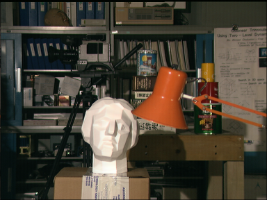
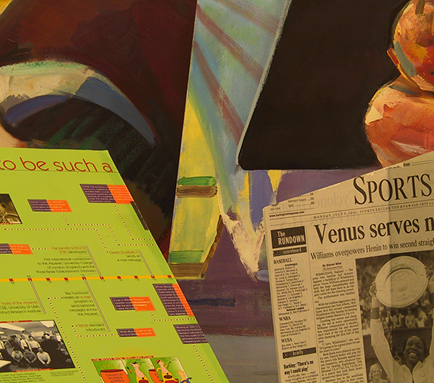
Execute the following command to execute a simulation of the accelerator using Verilator. It is worth noting that the images available for the evaluations are: Cones, Teddy, Tsukuba, and Venus.
# the first time you run the simulation you need to enable the conversion from VHDL to verilog using -gv 1 flag
python run_stereo_simulation_tb.py -im Cones -gv 1
# if you already generated the Stereo_Match.v file, you can launch the simulation as follows
python run_stereo_simulation_tb.py -im Cones
Using cocotb + verilator
We also provide support for Python-based testbench simulation using cocotb plus Verilator. To enable this simulation you can execute the following commands:
# the first time you run the simulation you need to enable the conversion from VHDL to verilog using -gv 1 flag
python run_stereo_simulation_tb.py -im Cones -simt cocotb+verilator -gv 1
# if you already generated the Stereo_Match.v file, you can launch the simulation as follows
python run_stereo_simulation_tb.py -im Cones -simt cocotb+verilator
Modelsim + Verilog files
Alternatively, we created the scripts that automatically execute the simulation using Modelsim of the verilog files generated by yosys+ghdl from the original VHDL design. To enable this simulation you can execute the following commands:
# the first time you run the simulation you need to enable the conversion from VHDL to verilog using -gv 1 flag
python run_stereo_simulation_tb.py -im Cones -simt qsim+verilog -gv 1
# if you already generated the Stereo_Match.v file, you can launch the simulation as follows
python run_stereo_simulation_tb.py -im Cones -simt qsim+verilog
Modelsim + VHDL files
Finally, you can simulate directly the VHDL design in Modelsim by executing the following commands:
# In this case there is no need to enable the verilog generation
python run_stereo_simulation_tb.py -im Cones -simt qsim+VHDL
3. Results visualization
After executing the simulation scripts, you must wait some time to get the accelerator results. It is expected that the VHDL -> verilog transformation take some minutes. However, after these steps, the simulations using Verilator are pretty fast, approx. 1 minute. On the other hand, when using Modelsim the VHDL simulation takes around 3 minutes and the Verilog simulation takes around 30 minutes, these are results obtained from a server with 256 cores and 128GB RAM.
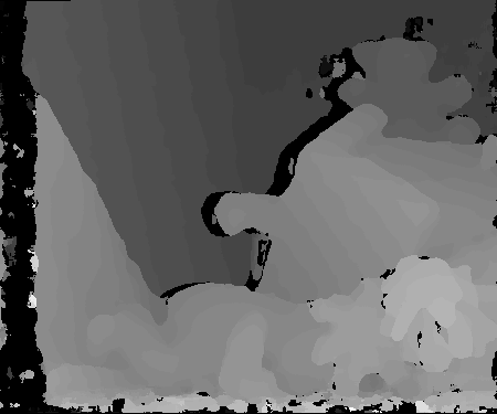
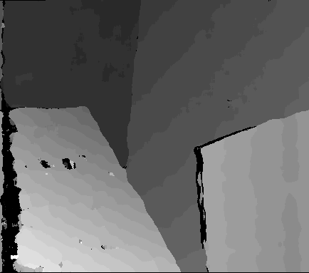
When the simulation ends, you will obtain a new image called Disparity_map.png, which shows the accelerator results. This image is converted into a grayscale format so that the lighter colors represent objects closer to the cameras, and darker colors belong to objects located further in the scene or undefined objects.
| Image | Left Image | Right Image | Output Result in grayscale |
| Tsukuba | 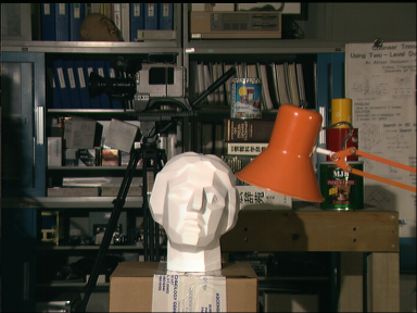 |
 |
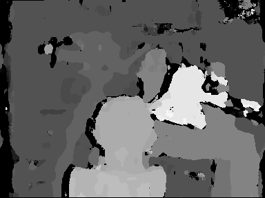 |
| Cones | 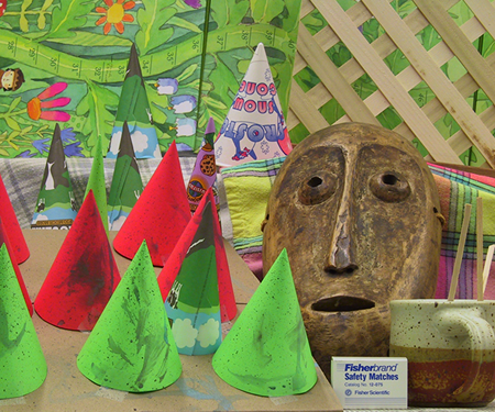 |
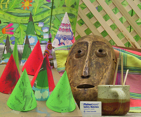 |
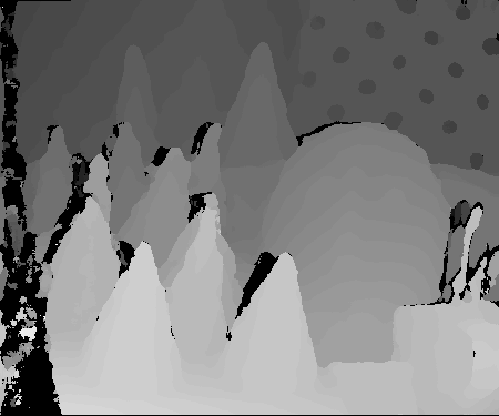 |
| Teddy | 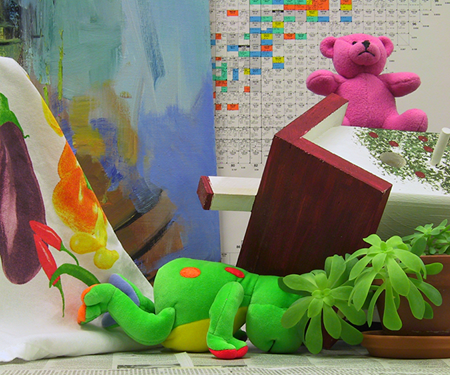 |
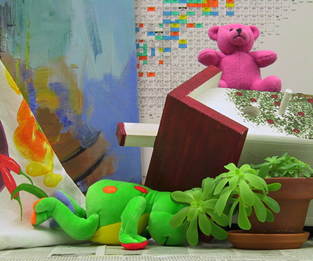 |
 |
| Venus | 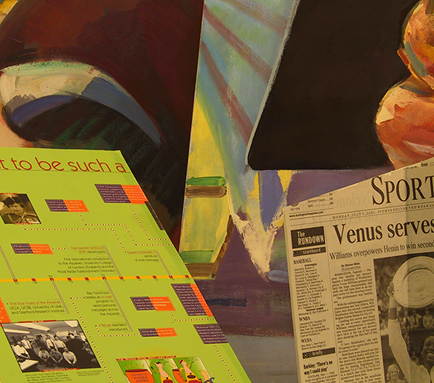 |
 |
 |
How to Cite?
  @software{Guerrero-Balaguera_SVC_2024,
    author = {Guerrero-Balaguera, Juan-David and Perez-Holguin, Wilson Javier},
    doi = {10.5281/zenodo.14033322},
    month = nov,
    title = {stereo vision core},
    url = {https://github.com/divadnauj-GB/stereo_vision_core},
    version = {1.0.0},
    year = {2024}
  }